July 2019 Was Not the Warmest on Record

Reblogged from Dr Roy Spencer.com:

August 2nd, 2019 by Roy W. Spencer, Ph. D.

July 2019 was probably the 4th warmest of the last 41 years. Global “reanalysis” datasets need to start being used for monitoring of global surface temperatures.

[NOTE: It turns out that the WMO, which announced July 2019 as a near-record, relies upon the ERA5 reanalysis which apparently departs substantially from the CFSv2 reanalysis, making my proposed reliance on only reanalysis data for surface temperature monitoring also subject to considerable uncertainty].

We are now seeing news reports (e.g. CNN, BBC, Reuters) that July 2019 was the hottest month on record for global average surface air temperatures.

One would think that the very best data would be used to make this assessment. After all, it comes from official government sources (such as NOAA, and the World Meteorological Organization [WMO]).

But current official pronouncements of global temperature records come from a fairly limited and error-prone array of thermometers which were never intended to measure global temperature trends. The global surface thermometer network has three major problems when it comes to getting global-average temperatures:

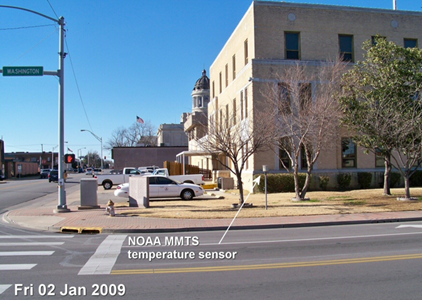
(1) The urban heat island (UHI) effect has caused a gradual warming of most land thermometer sites due to encroachment of buildings, parking lots, air conditioning units, vehicles, etc. These effects are localized, not indicative of most of the global land surface (which remains most rural), and not caused by increasing carbon dioxide in the atmosphere. Because UHI warming “looks like” global warming, it is difficult to remove from the data. In fact, NOAA’s efforts to make UHI-contaminated data look like rural data seems to have had the opposite effect. The best strategy would be to simply use only the best (most rural) sited thermometers. This is currently not done.

(2) Ocean temperatures are notoriously uncertain due to changing temperature measurement technologies (canvas buckets thrown overboard to get a sea surface temperature sample long ago, ship engine water intake temperatures more recently, buoys, satellite measurements only since about 1983, etc.)

(3) Both land and ocean temperatures are notoriously incomplete geographically. How does one estimate temperatures in a 1 million square mile area where no measurements exist?

There’s a better way.

A more complete picture: Global Reanalysis datasets

(If you want to ignore my explanation of why reanalysis estimates of monthly global temperatures should be trusted over official government pronouncements, skip to the next section.)

Various weather forecast centers around the world have experts who take a wide variety of data from many sources and figure out which ones have information about the weather and which ones don’t.

But, how can they know the difference? Because good data produce good weather forecasts; bad data don’t.

The data sources include surface thermometers, buoys, and ships (as do the “official” global temperature calculations), but they also add in weather balloons, commercial aircraft data, and a wide variety of satellite data sources.

Why would one use non-surface data to get better surface temperature measurements? Since surface weather affects weather conditions higher in the atmosphere (and vice versa), one can get a better estimate of global average surface temperature if you have satellite measurements of upper air temperatures on a global basis and in regions where no surface data exist. Knowing whether there is a warm or cold airmass there from satellite data is better than knowing nothing at all.

Furthermore, weather systems move. And this is the beauty of reanalysis datasets: Because all of the various data sources have been thoroughly researched to see what mixture of them provide the best weather forecasts
(including adjustments for possible instrumental biases and drifts over time), we know that the physical consistency of the various data inputs was also optimized.

Part of this process is making forecasts to get “data” where no data exists. Because weather systems continuously move around the world, the equations of motion, thermodynamics, and moisture can be used to estimate temperatures where no data exists by doing a “physics extrapolation” using data observed on one day in one area, then watching how those atmospheric characteristics are carried into an area with no data on the next day. This is how we knew there were going to be some exceeding hot days in France recently: a hot Saharan air layer was forecast to move from the Sahara desert into western Europe.

This kind of physics-based extrapolation (which is what weather forecasting is) is much more realistic than (for example) using land surface temperatures in July around the Arctic Ocean to simply guess temperatures out over the cold ocean water and ice where summer temperatures seldom rise much above freezing. This is actually one of the questionable techniques used (by NASA GISS) to get temperature estimates where no data exists.

If you think the reanalysis technique sounds suspect, once again I point out it is used for your daily weather forecast. We like to make fun of how poor some weather forecasts can be, but the objective evidence is that forecasts out 2-3 days are pretty accurate, and continue to improve over time.

The Reanalysis picture for July 2019

The only reanalysis data I am aware of that is available in near real time to the public is from WeatherBell.com, and comes from NOAA’s Climate Forecast System Version 2 (CFSv2).

The plot of surface temperature departures from the 1981-2010 mean for July 2019 shows a global average warmth of just over 0.3 C (0.5 deg. F) above normal:

Note from that figure how distorted the news reporting was concerning the temporary hot spells in France, which the media reports said contributed to global-average warmth. Yes, it was unusually warm in France in July. But look at the cold in Eastern Europe and western Russia. Where was the reporting on that? How about the fact that the U.S. was, on average, below normal?

The CFSv2 reanalysis dataset goes back to only 1979, and from it we find that July 2019 was actually cooler than three other Julys: 2016, 2002, and 2017, and so was 4th warmest in 41 years. And being only 0.5 deg. F above average is not terribly alarming.

Our UAH lower tropospheric temperature measurements had July 2019 as the third warmest, behind 1998 and 2016, at +0.38 C above normal.

Why don’t the people who track global temperatures use the reanalysis datasets?

The main limitation with the reanalysis datasets is that most only go back to 1979, and I believe at least one goes back to the 1950s. Since people who monitor global temperature trends want data as far back as possible (at least 1900 or before) they can legitimately say they want to construct their own datasets from the longest record of data: from surface thermometers.

But most warming has (arguably) occurred in the last 50 years, and if one is trying to tie global temperature to greenhouse gas emissions, the period since 1979 (the last 40+ years) seems sufficient since that is the period with the greatest greenhouse gas emissions and so when the most warming should be observed.

So, I suggest that the global reanalysis datasets be used to give a more accurate estimate of changes in global temperature for the purposes of monitoring warming trends over the last 40 years, and going forward in time. They are clearly the most physically-based datasets, having been optimized to produce the best weather forecasts, and are less prone to ad hoc fiddling with adjustments to get what the dataset provider thinks should be the answer, rather than letting the physics of the atmosphere decide.

GHCN V4 warming

Reblogged from Clive Best:

Posted on July 31, 2019 by Clive Best

In this post I investigate what has changed in global temperatures moving from GHCN-V3 to GHCN-V4, and in particular why V4 gives higher temperatures than V3  after 2000.

Whenever a new temperature series is released it inevitably shows an increase in recent warming, forever edging closer to  CMIP5 models.   The Hiatus in warming as reported in AR5,  has now completely vanished following regular “updates” to the HadCRUT4 temperatures since 2012.  Simultaneously model predictions have been edging downwards through a process of “blending” them to better fit the data. Ocean surface temperature data are now joining in to play their part in this warming process. The new HADSST4 corrections produces ~0.1C more warming than HADSST3, and the main reason for this is simply a change in the definition of the measurement depth of floating buoys. No doubt a new HadCRUT5 is now in the pipeline to complete the job. Of course nature itself doesn’t care less about how we measure the global temperature,  and the climate remains what it is. It is just the ‘interpretation’ of measurement data that is changing with time and this process seems to always increase recent temperatures. The world is warming by 10ths of a degree overnight as each new iteration is published. Now I have discovered that the latest GHCN V4  station data is continuing this trend as identified in the previous post. I have looked more deeply into why.

GHCNV4 has far more stations (27410) than V3 (7280) but turns out to be a completely new independent dataset. It is not an evolution of V3 even though it is called V4. GHCNV4 is 85% based on GHCN-Daily which is an NCDC archive of daily weather station records from around the world. V4 has no direct ancestry to V3 at all. Even the station ID numbering has been radically changed from that used in V3, making it almost impossible to track down any changes in station measurement data between V3 and V4. Despite that, I decided  to dig down a bit further.

About a year ago I actually studied GHCN-Daily using a 3D icosahedral grid to integrate the daily anomalies into annual anomalies.  In the end I got almost exactly the same result as CRUTEM4 for recent years after 1950, which  also agreed with the then GCHN V3. That implies that the data were then aligned with the results of both CRU and V3C. So something else has changed when moving data from GHCN-Daily to GHCN-V4.

So how is it possible that now V4 shows significantly more warming than V3 after 2002, when a year ago GHCN-Daily did not? Have the underlying station data been “corrected” yet again since V3C? To investigate this I used a convoluted method to identify only the V3 stations buried inside the V4 inventory by using their WMO IDs mapped through the GHCN-Daily directory. This procedure identified about half of  the 7280 versions of V3 stations, bearing in mind that V4 contains 24710 stations! The other half are not primary WMO stations. I then used my standard Spherical Triangulation algorithm to calculate annual global temperatures based only on these 3500 V4 versions of  V3 stations. If the underlying station temperatures were  the same as those in V3C then they should produce the same results as those from V3C.  Do they?

The results  are shown below.

Perhaps even more striking is the monthly agreement between the full V4C result and the V4 result restricted to 3500 V3 stations. The agreement is remarkably good. It should be compared to the V4 versus V3 comparison in the previous post.

So the answer to the question is no they do not agree with V3.  This must mean that the V4 versions of V3 station data are indeed different to those in the original V3 station data. So it is these changes that have caused the apparent increase in warming since 2004. The graphs above  show  that they are almost identical to the full  station results from V4C. It is also not true that somehow V4  has greater coverage in the Arctic and this can explain the increased warming over V3. The reason is simply that the underlying data have somehow been changed.

You get a different result from V4 and V3 using the same station data.

How Cold Air Caused a Heatwave

Reblogged from Watts Up With That:

Guest Blogger / June 26, 2019

Guest Post from Jim Steele

From What’s Natural? Column published in Pacifica Tribune June 26, 2019

 

I was recently asked if the record June 2019 heat in the San Francisco Bay Area validated CO₂ driven climate models. Surprisingly climate scientists have now demonstrated the heat wave was largely due to an intrusion of record cold air into the Pacific Northwest. How?

Basically, the winds’ direction controls the San Francisco Bay Area’s weather. In summer, California’s inland regions heat faster than the ocean, so the winds blow inland from the cooler ocean. Those onshore winds bring cooling fog, our natural air conditioner. Later, as the sun retreats southward in the fall, the land cools faster than the ocean. Seasonal winds then reverse and blow from the cooling land out to sea. Those winds keep the fog offshore. Without fog, San Franciscans finally enjoy pleasantly warm days in September and October. In northern California those strong offshore winds are called the Diablo winds. Although Diablo winds bring welcome warmth, those winds also increase wildfire danger.

Typically, inland California heats up in June drawing in the fog. But that temporarily changed when a surge of record cold air briefly entered Washington state and then moved down into northeastern California and Nevada. Dr. Cliff Mass, a climate scientist at the University of Washington, studies the Diablo winds. On his popular weather blog, he discussed how that intruding cold air created an unseasonal burst of Diablo winds that then kept the fog offshore. Without cooling fog, solar heating increased temperatures dramatically. According to Accuweather, San Francisco’s maximum temperature on Friday June 7^th was 67 °F, skyrocketed to a record 97 °F by Monday and then fell to 61 °F three days later as onshore winds returned.

Such rapid temperature change is never caused by a slowly changing greenhouse effect. Nevertheless, the media asks if rising CO₂ concentrations could have contributed to the higher temperatures or made the heatwave more likely?

Although definitions vary, the World Meteorological Organization defines a heat wave as 5 or more consecutive days of prolonged heat in which daily maximum temperatures are 9+ °F higher than average. Assuming the rise in CO₂ concentration increased all temperatures relative to the 20^th century average, it is believed maximum temperatures are more likely to exceed that 9 °F threshold. But heatwaves are not caused by increasing greenhouse gases.

The science is solid that greenhouse gases can intercept escaping heat and re-direct a portion of that heat back to earth. That downward directed heat reduces how quickly the earth cools, and thus the earth warms. However, heat waves typically occur when greenhouse gas concentrations are greatly reduced. Eighty percent or more of our greenhouse effect is caused not by CO₂, but by water vapor. Satellite data shows the dry conditions that accompany a heat wave actually reduce the greenhouse effect because drier air allows more infrared heat to escape back to space. However, like less fog, less water vapor and less clouds allow more solar heating. So despite the increase in escaping heat, increased solar heating dominates the weather and temperatures rise.

The important contribution of dryness to heat waves helps explain why the USA experienced its worst heat waves during the 1930s Dust Bowl years (see EPA Heatwave Index above). Furthermore, the EPA’s heat wave index appears totally independent of rising CO2 concentrations. Dryness also helps to explain why the hottest air temperature ever recorded anywhere in the world happened over a century ago in Death Valley on July 10, 1913; a time of much lower CO₂ concentrations.

To summarize, an intrusion of record cold air into the Pacific Northwest generated unseasonal Diablo winds in northern California. Those offshore winds prevented the fog from reaching and cooling the land. In addition, because the Diablo winds are abnormally dry, solar heating of the land increased. Those combined effects caused temperatures to temporarily jump by 30 °F.

Lastly, not only can Diablo winds cause heatwaves, Diablo winds will fan small fires into huge devastating infernos such as the one that destroyed Paradise, California. Fortunately, there were few wildfire ignitions during this heat wave. To be safe, Pacific Gas and Electric had shut off electricity to areas predicted to have high wind speeds. So Dr. Mass mused, that because colder temperatures generate the destructive Diablo winds, climate warming may have some benefits.

Jim Steele is retired director of the Sierra Nevada Field Campus, SFSU

and authored Landscapes and Cycles: An Environmentalist’s Journey to Climate Skepticism

Whatever happened to the Global Warming Hiatus?

Reblogged from Clive Best:

Posted on June 24, 2019 by Clive Best

The last IPCC assessment in 2013 showed a clear pause in global warming lasting 16 years from  1998 to 2012 – the notorious hiatus. As a direct consequence of this  AR5 estimates of climate sensitivity were reduced and CMIP5 models appeared to clearly overestimate trends. Following the first release of HadCRUT4 in 2014  the ‘headline’ then was that 2005 and 2010 were marginally warmer than 1998. This was the first dent in removing the hiatus. Since then each new version of H4 has showed further incremental warming trends, such that by 2019 the hiatus has now completely vanished. Anyone mentioning it today is likely to be ridiculed by the climate science community. So how did this reversal happen within just 5 years? I decided to find out exactly why the post 1998 temperature record changed so dramatically in such a short period of time.

In what follows I always use the same algorithm as CRU for the station data and then blend that with the Hadley SST data. I have checked that I can reproduce exactly the latest HadCRUT4.6 results based on the current 7820 stations from CRU merged with  HadSST3. Back in 2012 I downloaded the original station data from CRU –  CRUTEM3. I have also downloaded the latest CRUTEM4 station data.

Figure 1 compares the latest HadCRUT4.6 results with the last version of HadCRUT3.

I had assumed that the reason for the apparent trend change was because CRUTEM4 had added many new weather stations in the Arctic (removing some in S.America as well), while additionally the SST data had also been updated (HadSST2 moved to HADSST3). However, as I show below, my assumption simply isn’t true.

To investigate I recalculated a ‘modern’ version of HadCRUT3 by using only the original 4100 stations (used by CRUTEM3) from CRUTEM4 station data.  The list of these stations are defined here. I then merged these with  both the older HadSST2 and HADSST3 to derive annual global temperature anomalies. Figure 2 shows the result. I get almost exactly the same values as the full 7820 stations in HadCRUT4. It certainly does not reproduce HadCRUT3 !

This result provides two conclusions.

1. Modern CRUTEM3 stations give a different result to the original CRUTEM3 stations.
2. SST data is not responsible  for the difference between HadCRUT4 and HadCRUT3

To confirm point 1) I used exactly the same code to regenerate HadCRUT3 temperature series using the original CRUTEM3 station data as opposed to the ‘modern’ values based on CRUTEM4.

The original CRUTEM3 station data I had previously downloaded in 2012. These are combined with HADSST2 data. Now we see that  the agreement with the H3 annual temperatures is very good, and indeed reproduces the hiatus.

So the conclusion is very simple. The monthly temperature values in over 4000 CRUTEM3 stations have all been continuously changed, and it is these changes alone that have resulted in transforming the 16 year long hiatus in global warming into a rising temperature trend. Furthermore all these updates have only affected temperatures AFTER 1998! Temperatures before 1998 have hardly changed at all, which is the second requirement needed to eliminate the hiatus.

P.S. I am sure there are excellent arguments as to why pair-wise ‘homogenisation’ is wonderful but why then does it only affect data after 1998 ?

Our Urban “Climate Crisis”

Reblogged from Watts Up With That:

Guest Blogger / May 17, 2019

By Jim Steele

Published in Pacifica Tribune May 14, 2019

What’s Natural

Our Urban “Climate Crisis”

Based on a globally averaged statistic, some scientists and several politicians claim we are facing a climate crisis. Although it’s wise to think globally, organisms are never affected by global averages. Never! Organisms only respond to local conditions. Always! Given that weather stations around the globe only record local conditions, it is important to understand over one third of the earth’s weather stations report a cooling trend (i.e. Fig 4 below ) Cooling trends have various local and regional causes, but clearly, areas with cooling trends are not facing a “warming climate crisis”. Unfortunately, by averaging cooling and warming trends, the local factors affecting varied trends have been obscured.

It is well known as human populations grow, landscapes lose increasing amounts of natural vegetation, experience a loss of soil moisture and are increasingly covered by heat absorbing pavement and structures. All those factors raise temperatures so that a city’s downtown area can be 10°F higher than nearby rural areas. Despite urban areas representing less than 3% of the USA’s land surface, 82% of our weather stations are located in urbanized areas. This prompts critical thinkers to ask, “have warmer urbanized landscapes biased the globally averaged temperature?” (Arctic warming also biases the global average, but that dynamic must await a future article.)

Satellite data reveal that in forested areas the maximum surface temperatures are 36°F cooler than in grassy areas, and grassy areas’ maximum surface temperatures can be 36°F cooler than the unvegetated surfaces of deserts and cities. To appreciate the warming effects of altered landscapes, walk barefoot across a cool grassy lawn on a warm sunny day and then step onto a burning asphalt roadway.

In natural areas like Yosemite National Park, maximum air temperatures are cooler now than during the 1930s. In less densely populated and more heavily forested California, maximum air temperatures across the northern two thirds of the state have not exceeded temperatures of the 1930s. In contrast, recently urbanized communities in China report rapid warming of 3°F to 9°F in just 10 years, associated with the loss of vegetation.

Although altered urban landscapes undeniably raise local temperatures, some climate researchers suggest warmer urban temperatures do not bias the globally averaged warming trend. They argue warming trends in rural areas are similar to urbanized areas. So, they theorize a warmer global temperature is simply the result of a stronger greenhouse effect. However, such studies failed to analyze how changes in vegetation and wetness can similarly raise temperatures in both rural and urban areas. For example, researchers reported overgrazing had raised grassland temperatures 7°F higher compared to grassland that had not been grazed. Heat from asphalt will increase temperatures at rural weather stations just as readily as urban stations.

To truly determine the effects of climate change on natural habitats requires observing trends from tree ring data obtained from mostly pristine landscapes. Instrumental data are overwhelmingly measured in disturbed urbanized areas. Thus, the difference between instrumental and tree ring temperature trends can illustrate to what degree landscapes changes have biased natural temperature trends. And those trends are strikingly different!

The latest reconstructions of summer temperature trends from the best tree ring data suggest the warmest 30-year period happened between 1927 and 1956. After 1956, tree rings recorded a period of cooling that lowered global temperatures by over 1°F. In contrast, although tree rings and instrumental temperatures agreed up to 1950, the instrumental temperature trend, as presented in NASA graphs, suggests a temperature plateau from 1950 to 1970 and little or no cooling. So, are these contrasting trends the result of an increased urban warming effect offsetting natural cooling?

After decades of cooling, tree ring data recorded a global warming trend but with temperatures just now reaching a warmth that approaches the 1930s and 40s. In contrast, instrumental data suggests global temperatures have risen by more than 1°F above the 1940s. Some suggest tree rings have suddenly become insensitive to recent warmth? But the different warming trends are again better explained by a growing loss of vegetation and increasing areas covered by asphalt affecting temperatures measured by thermometers compared with temperatures determined from tree ring data in natural habitats.

Humans are increasingly inhabiting urban environments with 66% of humans projected to inhabit urban areas by 2030. High population densities typically reduce cooling vegetation, reduce wetlands and soil moisture, and increase landscape areas covered by heat retaining pavements. Thus, we should expect trends biased from urbanized landscapes to continue to rise. But there is a real solution to this “urban climate crisis.” It requires increasing vegetation, creating more parks and greenbelts, restoring wetlands and streams, and reducing heat absorbing pavements and roofs. Reducing CO₂ concentrations will not reduce stifling urban temperatures.

Jim Steele is the retired director of San Francisco State University’s Sierra Nevada Field Campus and authored Landscapes and Cycles: An Environmentalist’s Journey to Climate Skepticism.

Chinese UHI study finds 0.34C/century inflation effect on average temperature estimate.

Tallbloke's Talkshop

New study published by Springer today makes interesting reading. Phil Jones’ ears will be burning brightly.

Abstract:
Historical temperature records are often partially biased by the urban heat island (UHI) effect. However, the exact magnitude of these biases is an ongoing, controversial scientific question, especially in regions like China where urbanization has greatly increased in recent decades. Previous studies have mainly used statistical information and selected static population targets, or urban areas in a particular year, to classify urban-rural stations and estimate the influence of urbanization on observed warming trends. However, there is a lack of consideration for the dynamic processes of urbanization. The Beijing-Tianjin-Hebei (BTH), Yangtze River Delta (YRD), and Pearl River Delta (PRD) are three major urban agglomerations in China which were selected to investigate the spatiotemporal heterogeneity of urban expansion effects on observed warming trends in this study. Based on remote sensing (RS) data, urban area expansion…

View original post 149 more words

What’s Wrong With The Surface Temperature Record? Guest: Dr. Roger Pielke Sr.

Reblogged from Watts Up With That:

Anthony Watts / May 13, 2019

Dr. Roger Pielke Sr. joins [Anthony Watts] on a podcast to discuss the surface temperature record, the upcoming IPCC report, and climate science moving forward.

Dr. Roger Pielke Sr. explains how the Intergovernmental Panel on Climate Change (IPCC) is incorrectly explaining climate change to the media and public. Pielke highlights how the IPCC ignores numerous drivers of climate aside from CO2, leading to numerous factual inaccuracies in the IPCC reports.

Climate monitoring station in a parking lot at University of Arizona, Tucson

We also cover what is wrong with the surface temperature record – specifically why many temperature readings are higher than the actual temperature.

Available on Amazon at a special low price – click image

Pielke is currently a Senior Research Scientist in CIRES and a Senior Research Associate at the University of Colorado-Boulder in the Department of Atmospheric and Oceanic Sciences (ATOC) at the University of Colorado in Boulder (November 2005 -present). He is also an Emeritus Professor of Atmospheric Science at Colorado State University.

BIG NEWS – Verified by NOAA – Poor Weather Station Siting Leads To Artificial Long Term Warming

Sierra Foothill Commentary

Based on the data collected for the Surface Station Project and analysis papers describing the results, my friend Anthony Watts has been saying for years that “surface temperature measurements (and long term trends) have been affected by encroachment of urbanization on the placement of weather stations used to measure surface air temperature, and track long term climate.”

When Ellen and I traveled across the country in the RV we visited weather stations in the historical weather network and took photos of the temperature measurement stations and the surrounding environments.

Now, NOAA has validated Anthony’s findings — weather station siting can influence the surface station long temperature record. Here some samples that were taken by other volunteers :

Impacts of Small-Scale Urban Encroachment on Air Temperature Observations

Ronald D. Leeper, John Kochendorfer, Timothy Henderson, and Michael A. Palecki
https://journals.ametsoc.org/doi/10.1175/JAMC-D-19-0002.1

Abstract

A field experiment was performed in Oak Ridge, TN, with four…

View original post 248 more words

Climate data shows no recent warming in Antarctica, instead a slight cooling

Reblogged from Watts Up With That:

Anthony Watts / May 10, 2019

Below is a plot from a resource we have not used before on WUWT, “RIMFROST“. It depicts the average temperatures for all weather stations in Antarctica. Note that there is some recent cooling in contrast to a steady warming since about 1959.

Data and plot provided by http://rimfrost.no 

Contrast that with claims by Michael Mann, Eric Steig, and others who used statistical tricks to make Antarctica warm up. Fortunately, it wasn’t just falsified by climate skeptics, but rebutted in peer review too.

Data provided by http://rimfrost.no 

H/T to Kjell Arne Høyvik‏  on Twitter

ADDED:

No warming has occurred on the South Pole from 1978 to 2019 according to satellite data (UAH V6). The linear trend is flat!

Analysis of new NASA AIRS study: 80% of U.S. Warming has been at Night

Reblogged from Watts Up With That:

Guest Blogger / April 30, 2019

By Dr. Roy Spencer

I have previously addressed the NASA study that concluded the AIRS satellite temperatures “verified global warming trends“. The AIRS is an infrared temperature sounding instrument on the NASA Aqua satellite, providing data since late 2002 (over 16 years). All results in that study, and presented here, are based upon infrared measurements alone, with no microwave temperature sounder data being used in these products.

That reported study addressed only the surface “skin” temperature measurements, but the AIRS is also used to retrieve temperature profiles throughout the troposphere and stratosphere — that’s 99.9% of the total mass of the atmosphere.

Since AIRS data are also used to retrieve a 2 meter temperature (the traditional surface air temperature measurement height), I was curious why that wasn’t used instead of the surface skin temperature. Also, AIRS allows me to compare to our UAH tropospheric deep-layer temperature products.

So, I downloaded the entire archive of monthly average AIRS temperature retrievals on a 1 deg. lat/lon grid (85 GB of data). I’ve been analyzing those data over various regions (global, tropical, land, ocean). While there are a lot of interesting results I could show, today I’m going to focus just on the United States.

AIRS temperature trend profiles averaged over the contiguous United States, Sept. 2002 through March 2019. Gray represents an average of day and night. Trends are based upon monthly departures from the average seasonal cycle during 2003-2018. The UAH LT temperature trend (and it’s approximate vertical extent) is in violet, and NOAA surface air temperature trends (Tmax, Tmin, Tavg) are indicated by triangles. The open circles are the T2m retrievals, which appear to be less trustworthy than the Tskin retrievals.

Because the Aqua satellite observes at nominal local times of 1:30 a.m. and 1:30 p.m., this allows separation of data into “day” and “night”. It is well known that recent warming of surface air temperatures (both in the U.S. and globally) has been stronger at night than during the day, but the AIRS data shows just how dramatic the day-night difference is… keeping in mind this is only the most recent 16.6 years (since September 2002):

The AIRS surface skin temperature trend at night (1:30 a.m.) is a whopping +0.57 C/decade, while the daytime (1:30 p.m.) trend is only +0.15 C/decade. This is a bigger diurnal difference than indicated by the NOAA Tmax and Tmin trends (triangles in the above plot). Admittedly, 1:30 a.m. and 1:30 pm are not when the lowest and highest temperatures of the day occur, but I wouldn’t expect as large a difference in trends as is seen here, at least at night.

Furthermore, these day-night differences extend up through the lower troposphere, to higher than 850 mb (about 5,000 ft altitude), even showing up at 700 mb (about 12,000 ft. altitude).

This behavior also shows up in globally-averaged land areas, and reverses over the ocean (but with a much weaker day-night difference). I will report on this at some point in the future.

If real, these large day-night differences in temperature trends is fascinating behavior. My first suspicion is that it has something to do with a change in moist convection and cloud activity during warming. For instance more clouds would reduce daytime warming but increase nighttime warming. But I looked at the seasonal variations in these signatures and (unexpectedly) the day-night difference is greatest in winter (DJF) when there is the least convective activity and weakest in summer (JJA) when there is the most convective activity.

One possibility is that there is a problem with the AIRS temperature retrievals (now at Version 6). But it seems unlikely that this problem would extend through such a large depth of the lower troposphere. I can’t think of any reason why there would be such a large bias between day and night retrievals when it can be seen in the above figure that there is essentially no difference from the 500 mb level upward.

It should be kept in mind that the lower tropospheric and surface temperatures can only be measured by AIRS in the absence of clouds (or in between clouds). I have no idea how much of an effect this sampling bias would have on the results.

Finally, note how well the AIRS low- to mid-troposphere temperature trends match the bulk trend in our UAH LT product. I will be examining this further for larger areas as well.